One approach inspired by human learning is through better priors or a world model. Intuitively, a human while learning to drive doesn’t rely solely on trial-and-error, but constructs an internal model of the car and its dynamics. Precise motor control was a relatively recent development in mammals alongside internal modeling, and may be key towards learning effective motor control.

The success of combining planning and learning in Monte Carlo Tree Search (MCTS) approaches has been shown in AlphaZero. Famous successes with AlphaZero have been in games such as Chess and Go, where there is a clean reward signal, and the state space is discrete. However, real-world robotic control problems often have a continuous action space with the presence of continuous noise. Can AlphaZero be used for learning optimal low-level controls?

The problem

CartLatAccel is a simple 1D controls environment with added realistic noise and trajectory following. This task is a very simple, vectorized cart dynamics environment for testing RL driving controls.

First, we use an MCTS online planner on the simple continuous toy problem. Then, we use MCTS search to train a value and policy network. This approach is similar to RL methods such as PPO with an actor and value network, except our loss is now supervised from MCTS training. The search and learning no longer happen simultaneously, since we use a good search mechanism combined with a policy which is able to generalize and guide the search.

We experiment with on-policy MCTS and value net learning, combining both planning and learning to find the optimal car lateral control.

Online planning

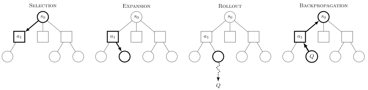
The first step was implementing vanilla MCTS for online planning. Online planning means before each step, we runm simulations from the current state and pick the best action which maximizes our expected returns Q(s,a). We modify MCTS to work with continuous action spaces. We can test this with a simple counting game where the goal is to get as close to 10 as possible and our actions are continuous from (-1,1).

For the simple CartLatAccel problem, we find that online MCTS (depth = 10, n_{sims} = 100) produced competitive results to a 32-layer MLP learned from PPO. MCTS achieved a reward of -3.81 compared to -3.45 using PPO running 100 steps.

AlphaZero for Continuous Control

We use the AlphaZero training procedure to learn a NN policy from MCTS. This can then be executed on a car without the need for real-time planning. We iteratively develop and test the value net and policy net with MCTS individually, before combining them into the final training.

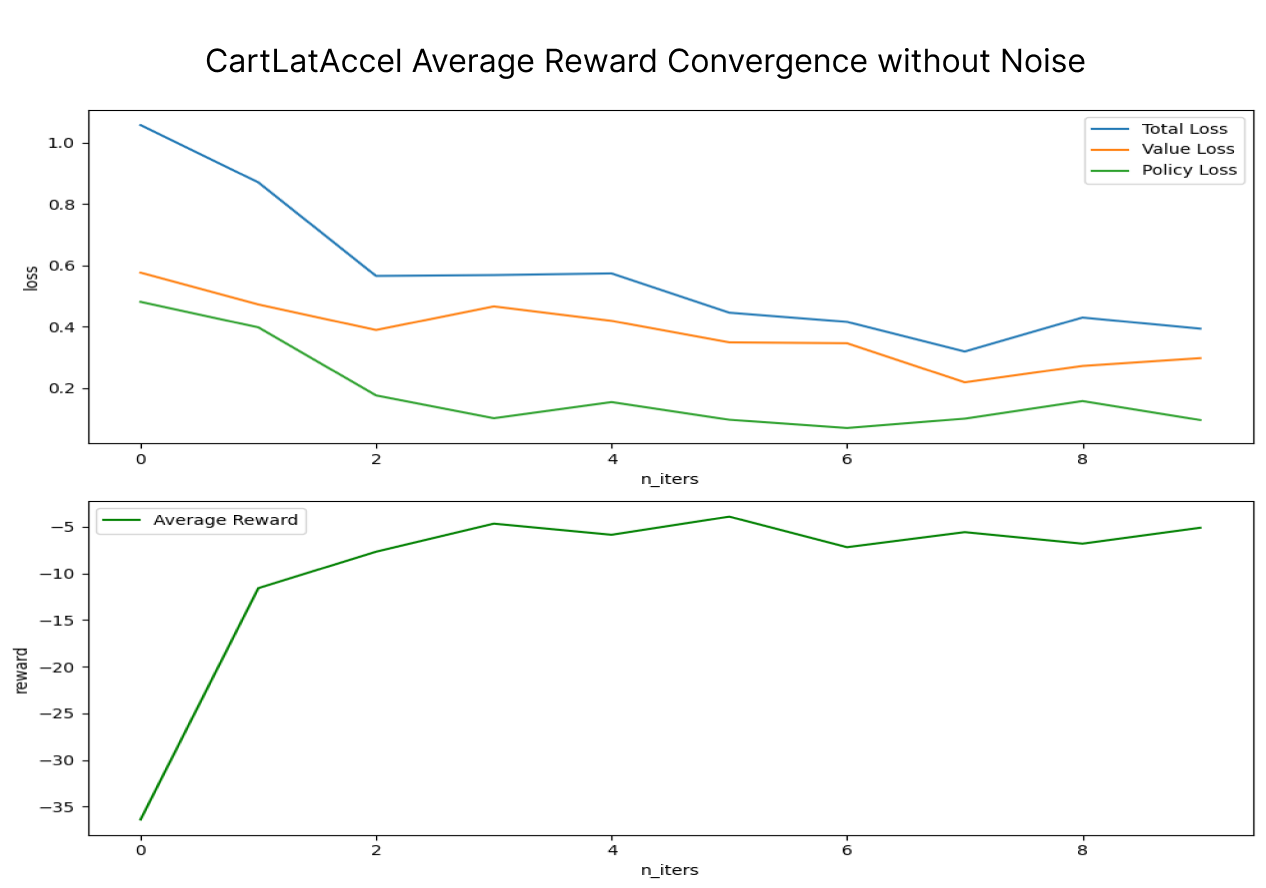
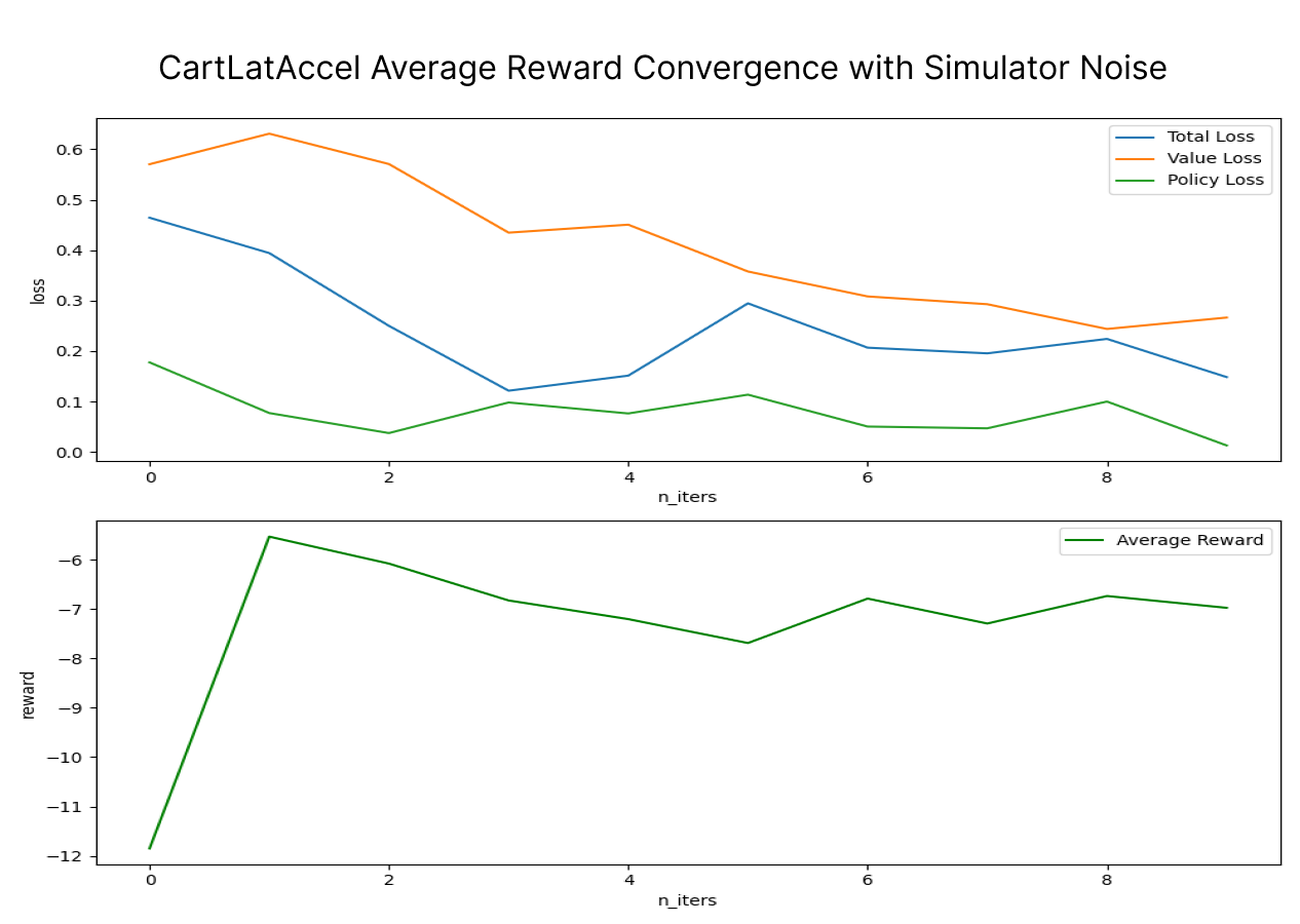
We find that AlphaZero beats PPO on the toy problem, achieving higher reward and lower variance of -5.52 (std 1.92) compared to -6.52 (std 2.44) over 10 evaluation runs. When noise is applied to the task, AlphaZero remains robust under noisy conditions (-6.52 std 2.44). Using MCTS helps lead to more reliable training targets, as it helps provide signal towards better simulated policies and stabilizes learning under noisy conditions. Learning and planning can find a more optimal solution, but is generally much slower, taking 200x longer for a similar number of steps.

Next steps

AlphaZero shows promising results on the controls task, achieving more stable learning and higher rewards than PPO. The next step is to apply AlphaZero to the controls challenge with more complex realistic noise. This is a much harder challenge and requires keeping track of intricate temporal correlations as context into the simulated car.

It’s unclear whether this approach will scale well to the challenge. However, if successful, we might find that the methods which led to the evolution of a grandmaster can also pave the way toward superhuman performance in autonomous driving. Combining planning and learning may be a step to useful autonomous robots capable of navigating the complexities of the real world.

He defines this concept of “hope”, which is really just expectation. We say we are hopeful when our advantage is positive.

He then goes on to show that this classic definition of expectation doesn’t match our common sense knowledge.

Consider a game² where you get paid $2 if the first H appears on the first toss, $4 if first H appears on the second, $8… so on. The expectation is infinite since the probabilities of H appearing on the nth toss is (1/2)^n, which means that the expectation is 1+1+… ad infinitum. Yet this is contrary to our common sense; nobody would pay an infinite amount to play this game.

So Laplace comes up with “moral hope” which, instead of taking the arithmetic mean in expectation, takes the geometric mean³. Intuitively if you have more fortune, the same profit means less to you; $100 is more valuable if you only have $10 vs if you have $1M. So moral expectation is function of both fortune and expected profit. It is the expected utility of the outcome rather than the net gain.

Most importantly, moral hope converges to a finite value for our game. Particularly, if you have $200, we should expect one to be willing to pay $8.71⁴.

This is both cool and useful - nonlinear expectation is currently how we model human behavior!⁵

If only SBF knew…

Consider a 2Nx2N lattice with 1 Ohm resistors on edges and a 1V battery on the diagonal of the center square. What is the current through the network? (equivalently, what is R_eq)

For N=1 case this is 1A (series and parallel resistors). For N=2 there are some clever tricks using symmetry, since you can join nodes of equipotential without changing the current flow and “fold” along the axis of symmetry, like folding a napkin in half. N=3 requires us to have a few more tricks up our sleeve, and can’t be resolved easily without Wye-Delta transforms. However,

There is no general closed form formula for current through a resistor lattice.¹

The difficult part is that order matters, and some operations aren’t reversible. Once you contract a node you break symmetry. You have to be smart about which ones to contract, replace, etc. so it’s the right shape. Topology matters.

There are many methods to approaching this, one is to represent circuits as graphs and an algorithm to apply the right operations in the right order². A more general method is to do tree search over possible actions on the graph. Some may formulate as random walk along nxn cartesian grid (since electrons are just random walking!)³

A circuit is just a graph with a set of simple linear constraints. Ohm’s law and KVL/KCL are all you really need to describe flow in a circuit. Yet from this problem we see that they are capable of expressing complex non-linear functions. It’s surprising how we often think of generality in NN but this is also paralleled in hardware. Circuits run our computer chips, power GPU clusters, control the electrical grid, and command the world’s electrons (and can also prove the AM-GM inequality⁴).

circuits: linear rules (Ohm’s law, KCL/KVL). It’s amazing to be surrounded by machines of such generality power.

nn: linear maps (matmul) + non-linear activations

Both circuits and NNs can be viewed as universal computational systems. Circuits are Turing complete digital simulators, NNs are universal function approximators. It’s amazing to be surrounded by machines of such generality.

A cool property of ML is that we can interpret the logits, outputs of the model, as anything we want. This leads to all sorts of rich interpretations.

Well, almost anything. The interpretations from logits don’t actually come from thin air, but derived from a few simple assumptions about the prior distribution and linear relationship. So from here our interpretation of logits, and our subsequent choice of estimator function, actually make sense!

Here, we’ll derive the equations for generalized linear models (GLMs), which form the foundation of classical ML/supervised learning.

Exponential family

To derive the family of GLMs, we first need to define the exponential family. A distribution is part of GLM if it can be written into following form:

This equation makes sense if you think about it in terms of Gaussian/Normal dist (verify for yourself that it looks similar). \(a(n)\) is normalization factor to make the area under the curve 1, for Gaussian it is \(\frac{1}{\sqrt{ 2\pi }}\), \(\eta\) is natural parameter, \(T(y)\) is the sufficient statistic and normally set to \(y\), \(b(y)\) is some term which doesn’t depend on \(\eta\).

Constructing GLMs

Assume prior probability -> what is the estimator? Give me any prior (ex. Gaussian) and I should be able to give you the respective classifier which operates under this assumption.

1. Distribution: \(y\vert x;\theta\), the prior distribution of y, is part of Exponential family (ex. Gaussian priors)
2. Linear relationship: The natural parameter \(\eta\) is related linearly with \(x\), \(\eta=\theta^{\top}x\)

Recall that in regression we want to predict the mean \(\mu\) (more precisely \(E[y\vert x]\)). In classification we want to minimize NLL (equivalent to MLE)

1. Write probability distribution in Exponential Family form \(p(y;\eta)\)
2. Find \(\eta\) (and optionally other parameters) in terms of \(\mu\), the mean of the probability distribution
3. Invert to solve for \(\mu\) in terms of \(\eta\). This is your canonical response function

For example, say I give you a dataset X and want you to predict the expected count y (e.g. X is weather/day of week…, y is how many customers you’ll see. Lots of processes for waiting time / counts are Poisson processes!). The Poisson distribution is \(p(y; \lambda) = \frac{e^{-\lambda}\lambda^y}{y!}\) \(\eta=\log(\lambda)\) so our mean we are predicting isis \(\lambda=e^\eta\) (verify this by putting it in exponential family form). So given X, you will output counts \(y=e^{\theta^{\top}X}\) and optimize for \(\theta\). This has a nice interpretation because, recalling our familiar softmax \(\frac{e^{z_{i}}}{\sum_{j}e^{z_{j}}}\), we have resp. prob = prob / total prob = counts / total counts. The poisson regression is just the numerator of the sigmoid, which is the expected counts! We’ve just discovered the Poisson regression.

Summary

You can do this for each distribution¹ to get the following mapping from distribution to estimator model. Here are a few common ones:

• Bernoulli => logistic/sigmoid \(\mu=\phi=\sigma(\eta)=\frac{1}{1+e^{-\eta}}\)
• Multinomial => softmax \(\frac{e^{\eta_{i}}}{\sum_{j}e^{\eta_{j}}}\)
• Gaussian => ordinary least squares \(\mu=\eta\) so predict \(y=\theta^{\top}X\)

Note: called OLS because the loss function is least squares \((y-\hat{y})^2\)

GLMs have quite a few other nice properties, such as being convex in terms of model parameters \(\theta\) (so the local minimum is the global minimum, and we have convergence guarantees for supervised learning), as well as having easy mean and variance calculations based on derivative \(a’(\eta)\). This deserves another discussion on its own², but it’s cool to see how a general family of functions with these properties can solve all sorts of problems in ML.

• What should you be optimizing for?
• How do you plan your future?
• What classes should I take? (useful vs fun?)
• How do I choose what person I want to be?

why you shouldn’t be able to predict their future

You can’t predict your future. Those who know with certainty are making a bet on themselves. This is only justified if you know enough about yourself in order to do so.¹

then what should I do?

Life is a multi-armed bandit problem. Most optimal policy is to explore first, then exploit. Right now I’m learning how to think, so I don’t care about the direct applications. Later on it’s always easy to apply knowledge or creativity, as long as you know what to look for.

You’ll never know what you could have fallen in love with. Henrik Karlsson writes “doggedly looking for what makes you feel alive”²

Keep dialing down temperature.

Pretrain, then finetune. Good foundation models beat out narrow AI.

Create a good model of the world first. Then apply it. Similar to the adage “to become a good artist, first develop good eye then just draw what you see”.

Exploring, but do so with intention. Pick something, go as deep as you can in it, then as soon as you realize it’s not for you, switch. Have a policy to explore the search space efficiently.

Once I understand myself better, I can better apply myself.